Narrate section
Modeling light with rays
Modeling light plays a crucial role in describing events based on light and helps designing mechanisms based on light (e.g., Realistic graphics in a video game, display or camera). This chapter introduces the most basic description of light using geometric rays, also known as raytracing. Raytracing has a long history, from ancient times to current Computer Graphics. Here, we will not cover the history of raytracing. Instead, we will focus on how we implement simulations to build "things" with raytracing in the future. As we provide algorithmic examples to support our descriptions, readers should be able to simulate light on their computers using the provided descriptions.
Are there other good resources on modeling light with rays?
When I first started coding Odak, the first paper I read was on raytracing. Thus, I recommend that paper for any starter:
- Spencer, G. H., and M. V. R. K. Murty. "General ray-tracing procedure." JOSA 52, no. 6 (1962): 672-678. 1
Beyond this paper, there are several resources that I can recommend for curious readers:
Ray description 
Informative · Practical
We have to define what "a ray" is. A ray has a starting point in Euclidean space (\(x_0, y_0, z_0 \in \mathbb{R}\)). We also have to define direction cosines to provide the directions for rays. Direction cosines are three angles of a ray between the XYZ axis and that ray (\(\theta_x, \theta_y, \theta_z \in \mathbb{R}\)). To calculate direction cosines, we must choose a point on that ray as \(x_1, y_1,\) and \(z_1\) and we calculate its distance to the starting point of \(x_0, y_0\) and \(z_0\):
Then, we can also calculate the Euclidian distance between starting point and the point chosen:
Thus, we describe each direction cosines as:
Now that we know how to define a ray with a starting point, \(x_0, y_0, z_0\) and a direction cosine, \(cos(\theta_x), cos(\theta_y), cos(\theta_z)\), let us carefully analyze the parameters, returns, and source code of the provided two following functions in odak dedicated to creating a ray or multiple rays.
Definition to create a ray.
Parameters:
-
xyz–List that contains X,Y and Z start locations of a ray. Size could be [1 x 3], [3], [m x 3]. -
abg–List that contains angles in degrees with respect to the X,Y and Z axes. Size could be [1 x 3], [3], [m x 3]. -
direction–If set to True, cosines of `abg` is not calculated.
Returns:
-
ray(tensor) –Array that contains starting points and cosines of a created ray. Size will be either [1 x 3] or [m x 3].
Source code in odak/learn/raytracing/ray.py
Definition to create a ray from two given points. Note that both inputs must match in shape.
Parameters:
-
x0y0z0–List that contains X,Y and Z start locations of a ray. Size could be [1 x 3], [3], [m x 3]. -
x1y1z1–List that contains X,Y and Z ending locations of a ray or batch of rays. Size could be [1 x 3], [3], [m x 3].
Returns:
-
ray(tensor) –Array that contains starting points and cosines of a created ray(s).
Source code in odak/learn/raytracing/ray.py
In the future, we must find out where a ray lands after a certain amount of propagation distance for various purposes, which we will describe in this chapter. For that purpose, let us also create a utility function that propagates a ray to some distance, \(d\), using \(x_0, y_0, z_0\) and \(cos(\theta_x), cos(\theta_y), cos(\theta_z)\):
Let us also check the function provided below to understand its source code, parameters, and returns. This function will serve as a utility function to propagate a ray or a batch of rays in our future simulations.
Definition to propagate a ray at a certain given distance.
Parameters:
-
ray–A ray with a size of [2 x 3], [1 x 2 x 3] or a batch of rays with [m x 2 x 3]. -
distance–Distance with a size of [1], [1, m] or distances with a size of [m], [1, m].
Returns:
-
new_ray(tensor) –Propagated ray with a size of [1 x 2 x 3] or batch of rays with [m x 2 x 3].
Source code in odak/learn/raytracing/ray.py
It is now time for us to put what we have learned so far into an actual code.
We can create many rays using the two functions, odak.learn.raytracing.create_ray_from_two_points and odak.learn.raytracing.create_ray.
However, to do so, we need to have many points in both cases.
For that purpose, let's carefully review this utility function provided below.
This utility function can generate grid samples from a plane with some tilt, and we can also define the center of our samples to position points anywhere in Euclidean space.
Generate samples over a surface.
Parameters:
-
no(list, default:[10, 10]) –Number of samples along each dimension.
-
size(list, default:[100.0, 100.0]) –Physical size of the surface along each dimension.
-
center(list, default:[0.0, 0.0, 0.0]) –Center location of the surface.
-
angles(list, default:[0.0, 0.0, 0.0]) –Tilt angles of the surface around X, Y, and Z axes.
Returns:
-
samples(tensor) –Generated samples.
-
rotx(tensor) –Rotation matrix around X axis.
-
roty(tensor) –Rotation matrix around Y axis.
-
rotz(tensor) –Rotation matrix around Z axis.
Source code in odak/learn/tools/sample.py
The below script provides a sample use case for the functions provided above. I also leave comments near some lines explaining the code in steps.
import sys
import odak
import torch  # (1)


def test(directory="test_output"):
    odak.tools.check_directory(directory)
    starting_point = torch.tensor([[5.0, 5.0, 0.0]])  # (2)
    end_points, _, _, _ = odak.learn.tools.grid_sample(
        no=[2, 2], size=[20.0, 20.0], center=[0.0, 0.0, 10.0]
    )  # (3)
    rays_from_points = odak.learn.raytracing.create_ray_from_two_points(
        starting_point, end_points
    )  # (4)

    starting_points, _, _, _ = odak.learn.tools.grid_sample(
        no=[3, 3],
        size=[100.0, 100.0],
        center=[0.0, 0.0, 10.0],
    )
    angles = torch.randn_like(starting_points) * 180.0  # (5)
    odak.learn.raytracing.create_ray(starting_points, angles)  # (6)

    distances = torch.ones(rays_from_points.shape[0]) * 12.5
    odak.learn.raytracing.propagate_ray(
        rays_from_points, distances
    )  # (7)

    visualize = False  # (8)
    if visualize:
        ray_diagram = odak.visualize.plotly.rayshow(line_width=3.0, marker_size=3.0)
        ray_diagram.add_point(starting_point, color="red")
        ray_diagram.add_point(end_points[0], color="blue")
        ray_diagram.add_line(starting_point, end_points[0], color="green")
        x_axis = starting_point.clone()
        x_axis[0, 0] = end_points[0, 0]
        ray_diagram.add_point(x_axis, color="black")
        ray_diagram.add_line(starting_point, x_axis, color="black", dash="dash")
        y_axis = starting_point.clone()
        y_axis[0, 1] = end_points[0, 1]
        ray_diagram.add_point(y_axis, color="black")
        ray_diagram.add_line(starting_point, y_axis, color="black", dash="dash")
        z_axis = starting_point.clone()
        z_axis[0, 2] = end_points[0, 2]
        ray_diagram.add_point(z_axis, color="black")
        ray_diagram.add_line(starting_point, z_axis, color="black", dash="dash")
        html = ray_diagram.save_offline()
        markdown_file = open("{}/ray.txt".format(directory), "w")
        markdown_file.write(html)
        markdown_file.close()
    assert True


if __name__ == "__main__":
    sys.exit(test())
- Required libraries are imported.
- Defining a starting point, in order X, Y and Z locations. Size of starting point could be s1] or [1, 1].
- Defining some end points on a plane in grid fashion.
odak.learn.raytracing.create_ray_from_two_pointsis verified with an example! Let's move on toodak.learn.raytracing.create_ray.- Creating starting points with
odak.learn.tools.grid_sampleand defining some angles as the direction usingtorch.randn. Note that the angles are in degrees. odak.learn.raytracing.create_rayis verified with an example!odak.learn.raytracing.propagate_a_rayis verified with an example!- Set it to
Trueto enable visualization.
The above code also has parts that are disabled (see visualize variable).
We disabled these lines intentionally to avoid running it at every run.
Let me talk about these disabled functions as well.
Odak offers a tidy approach to simple visualizations through packages called Plotly and kaleido.
To make these lines work by setting visualize = True, you must first install plotly in your work environment.
This installation is as simple as pip3 install plotly kaleido in a Linux system.
As you install these packages and enable these lines, the code will produce a visualization similar to the one below.
Note that this is an interactive visualization where you can interact with your mouse clicks to rotate, shift, and zoom.
In this visualization, we visualize a single ray (green line) starting from our defined starting point (red dot) and ending at one of the end_points (blue dot).
We also highlight three axes with black lines to provide a reference frame.
Although odak.visualize.plotly offers us methods to visualize rays quickly for debugging, it is highly suggested to stick to a low number of lines when using it (e.g., say not exceeding 100 rays in total).
The proper way to draw many rays lies in modern path-tracing renderers such as Blender.
How can I learn more about more sophisticated renderers like Blender?
Blender is a widely used open-source renderer that comes with sophisticated features.
It is user interface could be challenging for newcomers.
A blog post published by SIGGRAPH Research Career Development Committee offers a neat entry-level post titled Rendering a paper figure with Blender written by Silvia Sellán.
In addition to Blender, there are various renderers you may be happy to know about if you are curious about Computer Graphics.
Mitsuba 3 is another sophisticated rendering system based on a SIGGRAPH paper titled Dr.Jit: A Just-In-Time Compiler for Differentiable Rendering 4 from Wenzel Jakob.
If you know any other, please share it with the class so that they also learn more about other renderers.
Challenge: Blender meets Odak
In light of the given information, we challenge readers to create a new submodule for Odak.
Note that Odak has odak.visualize.blender submodule.
However, at the time of this writing, this submodule works as a server that sends commands to a program that has to be manually triggered inside Blender.
Odak seeks an upgrade to this submodule, where users can draw rays, meshes, or parametric surfaces easily in Blender with commands from Odak.
This newly upgraded submodule should require no manual processes.
To add these to odak, you can rely on the pull request feature on GitHub.
You can also create a new engineering note for your new submodule in docs/notes/odak_meets_blender.md.
Intersecting rays with surfaces 
Informative · Practical
Rays we have described so far help us explore light and matter interactions. Often in simulations, these rays interact with surfaces. In a simulation environment for optical design, equations often describe surfaces continuously. These surface equations typically contain a number of parameters for defining surfaces. For example, let us consider a sphere, which follows a standard equation as follows,
Where \(r\) represents the diameter of that sphere, \(x_0, y_0, z_0\) defines the center location of that sphere, and \(x, y, z\) are points on the surface of a sphere. When testing if a point is on a sphere, we use the above equation by inserting the point to be tested as \(x, y, z\) into that equation. In other words, to find a ray and sphere intersection, we must identify a distance that propagates our rays a certain amount and lends on a point on that sphere, and we can use the above sphere equation for identifying the intersection point of that rays. As long the surface equation is well degined, the same strategy can be used for any surfaces. In addition, if needed for future purposes (e.g., reflecting or refracting light off the surface of that sphere), we can also calculate the surface normal of that sphere by drawing a line by defining a ray starting from the center of that sphere and propagating towards the intersection point. Let us examine, how we can identify intersection points for a set of given rays and a sphere by examining the below function.
Definition to find the intersection between ray(s) and sphere(s).
Parameters:
-
ray–Input ray(s). Expected size is [1 x 2 x 3] or [m x 2 x 3]. -
sphere–Input sphere. Expected size is [1 x 4]. -
learning_rate–Learning rate used in the optimizer for finding the propagation distances of the rays. -
number_of_steps–Number of steps used in the optimizer. -
error_threshold–The error threshold that will help deciding intersection or no intersection.
Returns:
-
intersecting_ray(tensor) –Ray(s) that intersecting with the given sphere. Expected size is [n x 2 x 3], where n could be any real number.
-
intersecting_normal(tensor) –Normal(s) for the ray(s) intersecting with the given sphere Expected size is [n x 2 x 3], where n could be any real number.
Source code in odak/learn/raytracing/boundary.py
The odak.learn.raytracing.intersect_w_sphere function uses an optimizer to identify intersection points for each ray.
Instead, a function could have accomplished the task with a closed-form solution without iterating over the intersection test, which could have been much faster than the current function.
If you are curious about how to fix the highlighted issue, you may want to see the challenge provided below.
Let us examine how we can use the provided sphere intersection function with an example provided at the end of this subsection.
import sys
import odak
import torch


def test(output_directory="test_output"):
    odak.tools.check_directory(output_directory)
    starting_points, _, _, _ = odak.learn.tools.grid_sample(
        no=[5, 5], size=[3.0, 3.0], center=[0.0, 0.0, 0.0]
    )
    end_points, _, _, _ = odak.learn.tools.grid_sample(
        no=[5, 5], size=[0.1, 0.1], center=[0.0, 0.0, 5.0]
    )
    rays = odak.learn.raytracing.create_ray_from_two_points(starting_points, end_points)
    center = torch.tensor([[0.0, 0.0, 5.0]])
    radius = torch.tensor([[3.0]])
    sphere = odak.learn.raytracing.define_sphere(center=center, radius=radius)  # (1)
    intersecting_rays, intersecting_normals, _, check = (
        odak.learn.raytracing.intersect_w_sphere(rays, sphere)
    )

    visualize = False  # (2)
    if visualize:
        ray_diagram = odak.visualize.plotly.rayshow(line_width=3.0, marker_size=3.0)
        ray_diagram.add_point(rays[:, 0], color="blue")
        ray_diagram.add_line(
            rays[:, 0][check], intersecting_rays[:, 0], color="blue"
        )
        ray_diagram.add_sphere(sphere, color="orange")
        ray_diagram.add_point(intersecting_normals[:, 0], color="green")
        html = ray_diagram.save_offline()
        markdown_file = open("{}/ray.txt".format(output_directory), "w")
        markdown_file.write(html)
        markdown_file.close()
    assert True


if __name__ == "__main__":
    sys.exit(test())
- Here we provide an example use case for
odak.learn.raytracing.intersect_w_sphereby providing a sphere and a batch of sample rays. - Uncomment for running visualization.
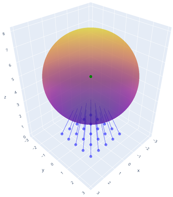
This section shows us how to operate with known geometric shapes, precisely spheres. However, not every shape could be defined using parametric modeling (e.g., nonlinearities such as discontinuities on a surface). We will look into another method in the next section, an approach used by folks working in Computer Graphics.
Challenge: Raytracing arbitrary surfaces
In light of the given information, we challenge readers to create a new function inside odak.learn.raytracing submodule that replaces the current intersect_w_sphere function.
In addition, the current unit test test/test_learn_raytracing_intersect_w_a_sphere.py has to adopt this new function.
odak.learn.raytracing submodule also needs new functions for supporting arbitrary surfaces (parametric).
New unit tests are needed to improve the submodule accordingly.
To add these to odak, you can rely on the pull request feature on GitHub.
You can also create a new engineering note for arbitrary surfaces in docs/notes/raytracing_arbitrary_surfaces.md.
Intersecting rays with meshes 
Informative · Practical
Parametric surfaces provide ease in defining shapes and geometries in various fields, including Optics and Computer Graphics.
However, not every object in a given scene could easily be described using parametric surfaces.
In many cases, including modern Computer Graphics, triangles formulate the smallest particle of an object or a shape.
These triangles altogether form meshes that define objects and shapes.
For this purpose, we will review source codes, parameters, and returns of three utility functions here.
We will first review odak.learn.raytracing.intersect_w_surface to understand how one can calculate the intersection of a ray with a given plane.
Later, we review odak.learn.raytracing.is_it_on_triangle function, which checks if an intersection point on a given surface is inside a triangle on that surface.
Finally, we will review odak.learn.raytracing.intersect_w_triangle function.
This last function combines both reviewed functions into a single function to identify the intersection between rays and a triangle.
Definition to find intersection point inbetween a surface and a ray. For more see: http://geomalgorithms.com/a06-_intersect-2.html
Parameters:
-
ray–A vector/ray. -
points–Set of points in X,Y and Z to define a planar surface.
Returns:
-
normal(tensor) –Surface normal at the point of intersection.
-
distance(float) –Distance in between starting point of a ray with it's intersection with a planar surface.
Source code in odak/learn/raytracing/boundary.py
Definition to check if a given point is inside a triangle. If the given point is inside a defined triangle, this definition returns True. For more details, visit: https://blackpawn.com/texts/pointinpoly/.
Parameters:
-
point_to_check–Point(s) to check. Expected size is [3], [1 x 3] or [m x 3]. -
triangle–Triangle described with three points. Expected size is [3 x 3], [1 x 3 x 3] or [m x 3 x3].
Returns:
-
result(tensor) –Is it on a triangle? Returns NaN if condition not satisfied. Expected size is [1] or [m] depending on the input.
Source code in odak/learn/raytracing/primitives.py
Definition to find intersection point of a ray with a triangle.
Parameters:
-
ray–A ray [1 x 2 x 3] or a batch of ray [m x 2 x 3]. -
triangle–Set of points in X,Y and Z to define a single triangle [1 x 3 x 3].
Returns:
-
normal(tensor) –Surface normal at the point of intersection with the surface of triangle. This could also involve surface normals that are not on the triangle. Expected size is [1 x 2 x 3] or [m x 2 x 3] depending on the input.
-
distance(float) –Distance in between a starting point of a ray and the intersection point with a given triangle. Expected size is [1 x 1] or [m x 1] depending on the input.
-
intersecting_ray(tensor) –Rays that intersect with the triangle plane and on the triangle. Expected size is [1 x 2 x 3] or [m x 2 x 3] depending on the input.
-
intersecting_normal(tensor) –Normals that intersect with the triangle plane and on the triangle. Expected size is [1 x 2 x 3] or [m x 2 x 3] depending on the input.
-
check(tensor) –A list that provides a bool as True or False for each ray used as input. A test to see is a ray could be on the given triangle. Expected size is [1] or [m].
Source code in odak/learn/raytracing/boundary.py
Using the provided utility functions above, let us build an example below that helps us find intersections between a triangle and a batch of rays.
import sys
import odak
import torch


def test(output_directory="test_output"):
    odak.tools.check_directory(output_directory)
    starting_points, _, _, _ = odak.learn.tools.grid_sample(
        no=[5, 5], size=[10.0, 10.0], center=[0.0, 0.0, 0.0]
    )
    end_points, _, _, _ = odak.learn.tools.grid_sample(
        no=[5, 5], size=[6.0, 6.0], center=[0.0, 0.0, 10.0]
    )
    rays = odak.learn.raytracing.create_ray_from_two_points(starting_points, end_points)
    triangle = torch.tensor([[[-5.0, -5.0, 10.0], [5.0, -5.0, 10.0], [0.0, 5.0, 10.0]]])
    normals, distance, _, _, check = odak.learn.raytracing.intersect_w_triangle(
        rays, triangle
    )  # (2)

    visualize = False  # (1)
    if visualize:
        ray_diagram = odak.visualize.plotly.rayshow(
            line_width=3.0, marker_size=3.0
        )  # (1)
        ray_diagram.add_triangle(triangle, color="orange")
        ray_diagram.add_point(rays[:, 0], color="blue")
        ray_diagram.add_line(rays[:, 0], normals[:, 0], color="blue")
        colors = []
        for color_id in range(check.shape[1]):
            if check[0, color_id]:
                colors.append("green")
            elif not check[0, color_id]:
                colors.append("red")
        ray_diagram.add_point(normals[:, 0], color=colors)
        html = ray_diagram.save_offline()
        markdown_file = open("{}/ray.txt".format(output_directory), "w")
        markdown_file.write(html)
        markdown_file.close()
    assert True


if __name__ == "__main__":
    sys.exit(test())
- Uncomment for running visualization.
- Returning intersection normals as new rays, distances from starting point of input rays and a check which returns True if intersection points are inside the triangle.
Why should we be interested in ray and triangle intersections?
Modern Computer Graphics uses various representations for defining three-dimensional objects and scenes. These representations include:
- Point Clouds: a series of XYZ coordinates from the surface of a three-dimensional object,
- Meshes: a soup of triangles that represents a surface of a three-dimensional object,
- Signed Distance Functions: a function informing about the distance between an XYZ point and a surface of a three-dimensional object,
- Neural Radiance Fields: A machine learning approach to learning ray patterns from various perspectives.
Historically, meshes have been mainly used to represent three-dimensional objects. Thus, intersecting rays and triangles are important for most Computer Graphics.
Challenge: Many triangles!
The example provided above deals with a ray and a batch of rays.
However, objects represented with triangles are typically described with many triangles but not one.
Note that odak.learn.raytracing.intersect_w_triangle deal with each triangle one by one, and may lead to slow execution times as the function has to visit each triangle one by one.
Given the information, we challenge readers to create a new function inside odak.learn.raytracing submodule named intersect_w_mesh.
This new function has to be able to work with multiple triangles (meshes) and has to be aware of "occlusions" (e.g., a triangle blocking another triangle).
In addition, a new unit test, test/test_learn_raytracing_intersect_w_mesh.py, has to adopt this new function.
To add these to odak, you can rely on the pull request feature on GitHub.
You can also create a new engineering note for arbitrary surfaces in docs/notes/raytracing_meshes.md.
Refracting and reflecting rays 
Informative · Practical
In the previous subsections, we reviewed ray intersection with various surface representations, including parametric (e.g., spheres) and non-parametric (e.g., meshes).
Please remember that raytracing is the most simplistic modeling of light.
Thus, often raytracing does not account for any wave or quantum-related nature of light.
To our knowledge, light refracts, reflects, or diffracts when light interfaces with a surface or, in other words, a changing medium (e.g., light traveling from air to glass).
In that case, our next step should be identifying a methodology to help us model these events using rays.
We compiled two utility functions that could help us to model a refraction or a reflection.
These functions are named odak.learn.raytracing.refract 1 and odak.learn.raytracing.reflect 1.
This first one, odak.learn.raytracing.refract follows Snell's law of refraction, while odak.learn.raytracing.reflect follows a perfect reflection case.
We will not go into details of this theory as its simplest form in the way we discuss it could now be considered common knowledge.
However, for curious readers, the work by Bell et al. 5 provides a generalized solution for the laws of refraction and reflection.
Let us carefully examine these two utility functions to understand their internal workings.
Definition to refract an incoming ray. Used method described in G.H. Spencer and M.V.R.K. Murty, "General Ray-Tracing Procedure", 1961.
Parameters:
-
vector–Incoming ray. Expected size is [2, 3], [1, 2, 3] or [m, 2, 3]. -
normvector–Normal vector. Expected size is [2, 3], [1, 2, 3] or [m, 2, 3]]. -
n1–Refractive index of the incoming medium. -
n2–Refractive index of the outgoing medium. -
error–Desired error.
Returns:
-
output(tensor) –Refracted ray. Expected size is [1, 2, 3]
Source code in odak/learn/raytracing/boundary.py
Definition to reflect an incoming ray from a surface defined by a surface normal. Used method described in G.H. Spencer and M.V.R.K. Murty, "General Ray-Tracing Procedure", 1961.
Parameters:
-
input_ray–A ray or rays. Expected size is [2 x 3], [1 x 2 x 3] or [m x 2 x 3]. -
normal–A surface normal(s). Expected size is [2 x 3], [1 x 2 x 3] or [m x 2 x 3].
Returns:
-
output_ray(tensor) –Array that contains starting points and cosines of a reflected ray. Expected size is [1 x 2 x 3] or [m x 2 x 3].
Source code in odak/learn/raytracing/boundary.py
Please note that we provide two refractive indices as inputs in odak.learn.raytracing.refract.
These inputs represent the refractive indices of two mediums (e.g., air and glass).
However, the refractive index of a medium is dependent on light's wavelength (color).
In the following example, where we showcase a sample use case of these utility functions, we will assume that light has a single wavelength.
But bear in mind that when you need to ray trace with lots of wavelengths (multi-color RGB or hyperspectral), one must ray trace for each wavelength (color).
Thus, the computational complexity of the raytracing increases dramatically as we aim growing realism in the simulations (e.g., describe scenes per color, raytracing for each color).
Let's dive deep into how we use these functions in an actual example by observing the example below.
import sys
import odak
import torch


def test(output_directory="test_output"):
    odak.tools.check_directory(output_directory)
    starting_points, _, _, _ = odak.learn.tools.grid_sample(
        no=[5, 5], size=[15.0, 15.0], center=[0.0, 0.0, 0.0]
    )
    end_points, _, _, _ = odak.learn.tools.grid_sample(
        no=[5, 5], size=[6.0, 6.0], center=[0.0, 0.0, 10.0]
    )
    rays = odak.learn.raytracing.create_ray_from_two_points(starting_points, end_points)
    triangle = torch.tensor([[[-5.0, -5.0, 10.0], [5.0, -5.0, 10.0], [0.0, 5.0, 10.0]]])
    normals, distance, intersecting_rays, intersecting_normals, check = (
        odak.learn.raytracing.intersect_w_triangle(rays, triangle)
    )
    n_air = 1.0  # (1)
    n_glass = 1.51  # (2)
    refracted_rays = odak.learn.raytracing.refract(
        intersecting_rays, intersecting_normals, n_air, n_glass
    )  # (3)
    reflected_rays = odak.learn.raytracing.reflect(
        intersecting_rays, intersecting_normals
    )  # (4)
    refract_distance = 11.0
    reflect_distance = 7.2
    propagated_refracted_rays = odak.learn.raytracing.propagate_ray(
        refracted_rays, torch.ones(refracted_rays.shape[0]) * refract_distance
    )
    propagated_reflected_rays = odak.learn.raytracing.propagate_ray(
        reflected_rays, torch.ones(reflected_rays.shape[0]) * reflect_distance
    )

    visualize = False
    if visualize:
        ray_diagram = odak.visualize.plotly.rayshow(
            columns=2,
            line_width=3.0,
            marker_size=3.0,
            subplot_titles=["Refraction example", "Reflection example"],
        )  # (1)
        ray_diagram.add_triangle(triangle, column=1, color="orange")
        ray_diagram.add_triangle(triangle, column=2, color="orange")
        ray_diagram.add_point(rays[:, 0], column=1, color="blue")
        ray_diagram.add_point(rays[:, 0], column=2, color="blue")
        ray_diagram.add_line(rays[:, 0], normals[:, 0], column=1, color="blue")
        ray_diagram.add_line(rays[:, 0], normals[:, 0], column=2, color="blue")
        ray_diagram.add_line(
            refracted_rays[:, 0],
            propagated_refracted_rays[:, 0],
            column=1,
            color="blue",
        )
        ray_diagram.add_line(
            reflected_rays[:, 0],
            propagated_reflected_rays[:, 0],
            column=2,
            color="blue",
        )
        colors = []
        for color_id in range(check.shape[1]):
            if check[0, color_id]:
                colors.append("green")
            elif not check[0, color_id]:
                colors.append("red")
        ray_diagram.add_point(normals[:, 0], column=1, color=colors)
        ray_diagram.add_point(normals[:, 0], column=2, color=colors)
        html = ray_diagram.save_offline()
        markdown_file = open("{}/ray.txt".format(output_directory), "w")
        markdown_file.write(html)
        markdown_file.close()
    assert True


if __name__ == "__main__":
    sys.exit(test())
- Refractive index of air (arbitrary and regardless of wavelength), the medium before the ray and triangle intersection.
- Refractive index of glass (arbitrary and regardless of wavelength), the medium after the ray and triangle intersection.
- Refraction process.
- Reflection process.
Challenge: Diffracted intefering rays
This subsection covered simulating refraction and reflection events.
However, diffraction or interference 6 is not introduced in this raytracing model.
This is because diffraction and interference would require another layer of complication.
In other words, rays have to have an extra dimension beyond their starting points and direction cosines, and they also have to have the quality named phase of light.
This fact makes a typical ray have dimensions of [1 x 3 x 3] instead of [1 x 2 x 3], where only direction cosines and starting points are defined.
Given the information, we challenge readers to create a new submodule, odak.learn.raytracing.diffraction, extending rays to diffraction and interference.
In addition, a new set of unit tests should be derived to adopt this new function submodule.
To add these to odak, you can rely on the pull request feature on GitHub.
You can also create a new engineering note for arbitrary surfaces in docs/notes/raytracing_diffraction_interference.md.
Optimization with rays
Informative · Practical
We learned about refraction, reflection, rays, and surface intersections in the previous subsection. We didn't mention it then, but these functions are differentiable 7. In other words, a modern machine learning library can keep a graph of a variable passing through each one of these functions (see chain rule). This differentiability feature is vital because differentiability makes our simulations for light with raytracing based on these functions compatible with modern machine learning frameworks such as Torch. In this subsection, we will use an off-the-shelf optimizer from Torch to optimize variables in our ray tracing simulations. In the first example, we will see that the optimizer helps us define the proper tilt angles for a triangle-shaped mirror and redirect light from a point light source towards a given target. Our first example resembles a straightforward case for optimization by containing only a batch of rays and a single triangle. The problem highlighted in the first example has a closed-form solution, and using an optimizer is obviously overkill. We want our readers to understand that the first example is a warm-up scenario where our readers understand how to interact with race and triangles in the context of an optimization problem. In our following second example, we will deal with a more sophisticated case where a batch of rays arriving from a point light source bounces off a surface with multiple triangles in parentheses mesh and comes at some point in our final target plane. This time we will ask our optimizer to optimize the shape of our triangles so that most of the light bouncing off there's optimized surface ends up at a location close to a target we define in our simulation. This way, we show our readers that a more sophisticated shape could be optimized using our framework, Odak. In real life, the second example could be a lens or mirror shape to be optimized. More specifically, as an application example, it could be a mirror or a lens that focuses light from the Sun onto a solar cell to increase the efficiency of a solar power system, or it could have been a lens helping you to focus on a specific depth given your eye prescription. Let us start from our first example and examine how we can tilt the surfaces using an optimizer, and in this second example, let us see how an optimizer helps us define and optimize shape for a given mesh.
import sys
import odak
import torch
from tqdm import tqdm


def test(
    output_directory="test_output",
    header="test_learn_raytracing_optimization.py",
):
    odak.tools.check_directory(output_directory)
    final_surface = torch.tensor(
        [[[-5.0, -5.0, 0.0], [5.0, -5.0, 0.0], [0.0, 5.0, 0.0]]]
    )
    final_target = torch.tensor([[3.0, 3.0, 0.0]])
    triangle = torch.tensor([[-5.0, -5.0, 10.0], [5.0, -5.0, 10.0], [0.0, 5.0, 10.0]])
    starting_points, _, _, _ = odak.learn.tools.grid_sample(
        no=[5, 5], size=[1.0, 1.0], center=[0.0, 0.0, 0.0]
    )
    end_point = odak.learn.raytracing.center_of_triangle(triangle)
    rays = odak.learn.raytracing.create_ray_from_two_points(starting_points, end_point)
    angles = torch.zeros(1, 3, requires_grad=True)
    learning_rate = 2e-1
    optimizer = torch.optim.Adam([angles], lr=learning_rate)
    loss_function = torch.nn.MSELoss()
    number_of_steps = 100
    t = tqdm(range(number_of_steps), leave=False, dynamic_ncols=True)
    for step in t:
        optimizer.zero_grad()
        rotated_triangle, _, _, _ = odak.learn.tools.rotate_points(
            triangle, angles=angles, origin=end_point
        )
        _, _, intersecting_rays, intersecting_normals, check = (
            odak.learn.raytracing.intersect_w_triangle(rays, rotated_triangle)
        )
        reflected_rays = odak.learn.raytracing.reflect(
            intersecting_rays, intersecting_normals
        )
        final_normals, _ = odak.learn.raytracing.intersect_w_surface(
            reflected_rays, final_surface
        )
        if step == 0:
            start_rays = rays.detach().clone()
            start_rotated_triangle = rotated_triangle.detach().clone()
            start_intersecting_rays = intersecting_rays.detach().clone()
            start_intersecting_normals = intersecting_normals.detach().clone()
            start_final_normals = final_normals.detach().clone()
        final_points = final_normals[:, 0]
        target = final_target.repeat(final_points.shape[0], 1)
        loss = loss_function(final_points, target)
        loss.backward(retain_graph=True)
        optimizer.step()
        t.set_description("Loss: {}".format(loss.item()))
    odak.log.logger.info(
        "{} -> Loss: {}, angles: {}".format(header, loss.item(), angles)
    )

    visualize = False
    if visualize:
        ray_diagram = odak.visualize.plotly.rayshow(
            columns=2,
            line_width=3.0,
            marker_size=3.0,
            subplot_titles=[
                "Surace before optimization",
                "Surface after optimization",
                "Hits at the target plane before optimization",
                "Hits at the target plane after optimization",
            ],
        )
        ray_diagram.add_triangle(start_rotated_triangle, column=1, color="orange")
        ray_diagram.add_triangle(rotated_triangle, column=2, color="orange")
        ray_diagram.add_point(start_rays[:, 0], column=1, color="blue")
        ray_diagram.add_point(rays[:, 0], column=2, color="blue")
        ray_diagram.add_line(
            start_intersecting_rays[:, 0],
            start_intersecting_normals[:, 0],
            column=1,
            color="blue",
        )
        ray_diagram.add_line(
            intersecting_rays[:, 0], intersecting_normals[:, 0], column=2, color="blue"
        )
        ray_diagram.add_line(
            start_intersecting_normals[:, 0],
            start_final_normals[:, 0],
            column=1,
            color="blue",
        )
        ray_diagram.add_line(
            start_intersecting_normals[:, 0],
            final_normals[:, 0],
            column=2,
            color="blue",
        )
        ray_diagram.add_point(final_target, column=1, color="red")
        ray_diagram.add_point(final_target, column=2, color="green")
        html = ray_diagram.save_offline()
        markdown_file = open("{}/ray.txt".format(output_directory), "w")
        markdown_file.write(html)
        markdown_file.close()
    assert True


if __name__ == "__main__":
    sys.exit(test())
Let us also look into the more sophisticated second example, where a triangular mesh is optimized to meet a specific demand, redirecting rays to a particular target.
import sys
import odak
import torch
from tqdm import tqdm


def test(
    output_directory="test_output",
    header="test/test_learn_raytracing_mesh.py",
):
    odak.tools.check_directory(output_directory)
    device = torch.device("cpu")
    final_target = torch.tensor([-2.0, -2.0, 10.0], device=device)
    final_surface = odak.learn.raytracing.define_plane(point=final_target)
    mesh = odak.learn.raytracing.planar_mesh(
        size=torch.tensor([1.1, 1.1]),
        number_of_meshes=torch.tensor([9, 9]),
        device=device,
    )
    start_points, _, _, _ = odak.learn.tools.grid_sample(
        no=[11, 11], size=[1.0, 1.0], center=[2.0, 2.0, 10.0]
    )
    end_points, _, _, _ = odak.learn.tools.grid_sample(
        no=[11, 11], size=[1.0, 1.0], center=[0.0, 0.0, 0.0]
    )
    start_points = start_points.to(device)
    end_points = end_points.to(device)
    loss_function = torch.nn.MSELoss(reduction="sum")
    learning_rate = 2e-3
    optimizer = torch.optim.AdamW([mesh.heights], lr=learning_rate)
    rays = odak.learn.raytracing.create_ray_from_two_points(start_points, end_points)
    number_of_steps = 100
    t = tqdm(range(number_of_steps), leave=False, dynamic_ncols=True)
    for step in t:
        optimizer.zero_grad()
        triangles = mesh.get_triangles()
        reflected_rays, reflected_normals = mesh.mirror(rays)
        final_normals, _ = odak.learn.raytracing.intersect_w_surface(
            reflected_rays, final_surface
        )
        final_points = final_normals[:, 0]
        target = final_target.repeat(final_points.shape[0], 1)
        if step == 0:
            start_triangles = triangles.detach().clone()
            reflected_rays.detach().clone()
            final_normals.detach().clone()
        loss = loss_function(final_points, target)
        loss.backward(retain_graph=True)
        optimizer.step()
        description = "{} -> Loss: {}".format(header, loss.item())
        t.set_description(description)
    odak.log.logger.info(description)

    visualize = False
    if visualize:
        ray_diagram = odak.visualize.plotly.rayshow(
            rows=1,
            columns=2,
            line_width=3.0,
            marker_size=1.0,
            subplot_titles=["Before optimization", "After optimization"],
        )
        for triangle_id in range(triangles.shape[0]):
            ray_diagram.add_triangle(
                start_triangles[triangle_id], row=1, column=1, color="orange"
            )
            ray_diagram.add_triangle(
                triangles[triangle_id], row=1, column=2, color="orange"
            )
        html = ray_diagram.save_offline()
        markdown_file = open("{}/ray.txt".format(output_directory), "w")
        markdown_file.write(html)
        markdown_file.close()
    assert True


if __name__ == "__main__":
    sys.exit(test())
Challenge: Differentiable detector
In our examples, where we try bouncing light towards a fixed target, our target is defined as a single point along XYZ axes.
However, in many cases in Optics and Computer Graphics, we may want to design surfaces to resemble a specific distribution of intensities over a plane (e.g., a detector or a camera sensor).
For example, the work by Schwartzburg et al. 8 designs optical surfaces such that when light refracts, the distribution of these intensities forms an image at some target plane.
To be able to replicate such works with Odak, odak needs a detector that is differentiable.
This detector could be added as a class in the odak.learn.raytracing submodule, and a new unit test could be added as test/test_learn_detector.py.
To add these to odak, you can rely on the pull request feature on GitHub.
Rendering scenes
Informative · Practical
This section shows how one can use raytracing for rendering purposes in Computer Graphics. Note that the provided example is simple, aiming to introduce a newcomer to how raytracing could be used for rendering purposes. The example uses a single perspective camera and relies on a concept called splatting, where rays originate from a camera towards a scene. The scene is composed of randomly colored triangles, and each time a ray hits a random colored triangle, our perspective camera's corresponding pixel is painted with the color of that triangle. Let us review our simple example by reading the code and observing its outcome.
import sys
import odak
import torch


def test(output_directory="test_output"):
    odak.tools.check_directory(output_directory)
    final_surface_point = torch.tensor([0.0, 0.0, 10.0])
    odak.learn.raytracing.define_plane(point=final_surface_point)
    no = [500, 500]
    start_points, _, _, _ = odak.learn.tools.grid_sample(
        no=no, size=[10.0, 10.0], center=[0.0, 0.0, -10.0]
    )
    end_point = torch.tensor([0.0, 0.0, 0.0])
    rays = odak.learn.raytracing.create_ray_from_two_points(start_points, end_point)
    mesh = odak.learn.raytracing.planar_mesh(
        size=torch.tensor([10.0, 10.0]),
        number_of_meshes=torch.tensor([40, 40]),
        angles=torch.tensor([0.0, -70.0, 0.0]),
        offset=torch.tensor([-2.0, 0.0, 5.0]),
    )
    triangles = mesh.get_triangles()
    play_button = torch.tensor(
        [
            [
                [1.0, 0.5, 3.0],
                [0.0, 0.5, 3.0],
                [0.5, -0.5, 3.0],
            ]
        ]
    )
    triangles = torch.cat((play_button, triangles), dim=0)
    background_color = torch.rand(3)
    triangles_color = torch.rand(triangles.shape[0], 3)
    image = torch.zeros(rays.shape[0], 3)
    for triangle_id, triangle in enumerate(triangles):
        _, _, _, _, check = odak.learn.raytracing.intersect_w_triangle(rays, triangle)
        check = check.squeeze(0).unsqueeze(-1).repeat(1, 3)
        color = triangles_color[triangle_id].unsqueeze(0).repeat(check.shape[0], 1)
        image[check] = color[check] * check[check]
    image[image == [0.0, 0.0, 0]] = background_color
    image = image.view(no[0], no[1], 3)
    odak.learn.tools.save_image(
        "{}/image.png".format(output_directory), image, cmin=0.0, cmax=1.0
    )
    assert True


if __name__ == "__main__":
    sys.exit(test())
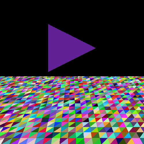
A modern raytracer used in gaming is far more sophisticated than the example we provide here. There aspects such as material properties or tracing the ray from its source to a camera or allowing rays to interface with multiple materials. Covering these aspects in a crash course like the one we provide here will take much work. Instead, we suggest our readers follow the resources provided in other classes, references provided at the end, or any other online available materials.
Conclusion
Informative
We can simulate light on a computer using various methods. We explain "raytracing" as one of these methods. Often, raytracing deals with light intensities, omitting many other aspects of light, like the phase or polarization of light. In addition, sending the right amount of rays from a light source into a scene in raytracing is always a struggle as an outstanding sampling problem. Raytracing creates many success stories in gaming (e.g., NVIDIA RTX or AMD Radeon Rays) and optical component design (e.g., Zemax or Ansys Speos).
Overall, we cover a basic introduction to how to model light as rays and how to use rays to optimize against a given target. Note that our examples resemble simple cases. This section aims to provide the readers with a suitable basis to get started with the raytracing of light in simulations. A dedicated and motivated reader could scale up from this knowledge to advance concepts in displays, cameras, visual perception, optical computing, and many other light-based applications.
Reminder
We host a Slack group with more than 300 members. This Slack group focuses on the topics of rendering, perception, displays and cameras. The group is open to public and you can become a member by following this link. Readers can get in-touch with the wider community using this public group.
-
GH Spencer and MVRK Murty. General ray-tracing procedure. JOSA, 52(6):672–678, 1962. ↩↩↩
-
Peter Shirley. Ray tracing in one weekend. Amazon Digital Services LLC, 1:4, 2018. ↩
-
Morgan McGuire. The graphics codex. 2018. ↩
-
Wenzel Jakob, Sébastien Speierer, Nicolas Roussel, and Delio Vicini. Dr. jit: a just-in-time compiler for differentiable rendering. ACM Transactions on Graphics (TOG), 41(4):1–19, 2022. ↩
-
Robert J Bell, Kendall R Armstrong, C Stephen Nichols, and Roger W Bradley. Generalized laws of refraction and reflection. JOSA, 59(2):187–189, 1969. ↩
-
Max Born and Emil Wolf. Principles of optics: electromagnetic theory of propagation, interference and diffraction of light. Elsevier, 2013. ↩
-
Adam Paszke, Sam Gross, Soumith Chintala, Gregory Chanan, Edward Yang, Zachary DeVito, Zeming Lin, Alban Desmaison, Luca Antiga, and Adam Lerer. Automatic differentiation in pytorch. NIPS 2017 Workshop Autodiff, 2017. ↩
-
Yuliy Schwartzburg, Romain Testuz, Andrea Tagliasacchi, and Mark Pauly. High-contrast computational caustic design. ACM Transactions on Graphics (TOG), 33(4):1–11, 2014. ↩