Narrate section
Computer-Generated Holography
In this section, we introduce Computer-Generated Holography (CGH) 1 as another emerging method to simulate light. CGH offers an upgraded but more computationally expensive way to simulating light concerning the raytracing method described in the previous section. This section dives deep into CGH and will explain how CGH differs from raytracing as we go.
What is holography?
Informative
Holography is a method in Optical sciences to represent light distribution using amplitude and phase of light. In much simpler terms, holography describes light distribution emitted from an object, scene, or illumination source over a surface by treating the light as a wave. The primary difference of holography concerning raytracing is that it accounts not only amplitude or intensity of light but also the phase of light. Unlike classical raytracing, holography also includes diffraction and interference phenomena. In raytracing, the smallest building block that defines light is a ray, whereas, in holography, the building block is a light distribution over surfaces. In other terms, while raytracing traces rays, holography deals with surface-to-surface light transfer.
Did you know this source?
There is an active repository on GitHub, where latest CGH papers relevant to display technologies are listed. Visit GitHub:bchao1/awesome-holography for more.
What is a hologram?
Informative
Hologram is either a surface or a volume that modifies the light distribution of incoming light in terms of phase and amplitude. Diffraction gratings, Holographic Optical Elements, or Metasurfaces are good examples of holograms. Within this section, we also use the term hologram as a means to describe a lightfield or a slice of a lightfield.
What is Computer-Generated Holography?
Informative
It is the computerized version (discrete sampling) of holography. In other terms, whenever you can program the phase or amplitude of light, this will get us to Computer-Generated Holography.
Where can I find an extensive summary on CGH?
You may be wondering about the greater physical details of CGH. In this case, we suggest our readers watch the video below. Please watch this video for an extensive summary on CGH 2.
Defining a slice of a lightfield 
Informative · Practical
CGH deals with generating optical fields that capture light from various scenes. CGH often describes these optical fields (a.k.a. lightfields, holograms) as planes. So in CGH, light travels from plane to plane, as depicted below. Roughly, CGH deals with plane to plane interaction of light, whereas raytracing is a ray or beam oriented description of light.
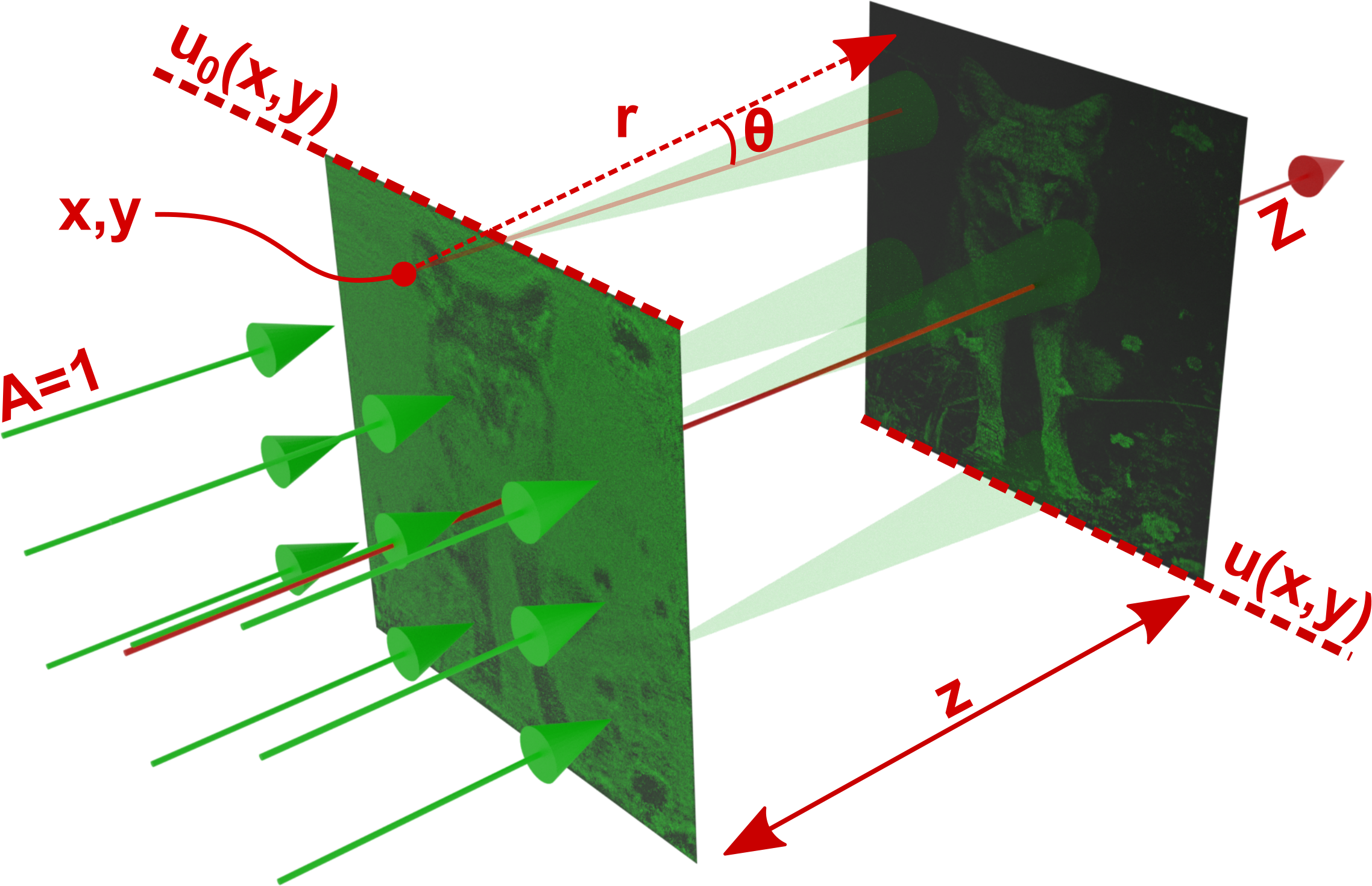
In other words, in CGH, you define everything as a "lightfield," including light sources, materials, and objects. Thus, we must first determine how to describe the mentioned lightfield in a computer. So that we can run CGH simulations effectively.
A lightfield is a planar slice in the context of CGH, as depicted in the above figure. This planar field is a pixelated 2D surface (could be represented as a matrix). The pixels in this 2D slice hold values for the amplitude of light, \(A\), and the phase of the light, \(\phi\) at each pixel. Whereas in classical raytracing, a ray only holds the amplitude or intensity of light. With a caveat, though, raytracing could also be made to care about the phase of light. Still, it will then arrive with all the complications of raytracing, like sampling enough rays or describing scenes accurately.
Each pixel in this planar lightfield slice encapsulates the \(A\) and \(\phi\) as \(A cos(wt + \phi)\). If you recall our description of light, we explain that light is an electromagnetic phenomenon. Here, we model the oscillating electric field of light with \(A cos(wt + \phi)\) shown in our previous light description. Note that if we stick to \(A cos(wt + \phi)\), each time two fields intersect, we have to deal with trigonometric conversion complexities like sampled in this example:
Where the indices zero and one indicate the first and second fields, and we have to identify the right trigonometric conversion to deal with this sum.
Instead of complicated trigonometric conversions, what people do in CGH is to rely on complex numbers as a proxy to these trigonometric conversions. In its proxy form, a pixel value in a field is converted into \(A e^{-j \phi}\), where \(j\) represents a complex number (\(\sqrt{-1}\)). Thus, with this new proxy representation, the same intersection problem we dealt with using sophisticated trigonometry before could be turned into something as simple as \(A_0 A_1 e^{-j(\phi_0 +\phi_1)}\).
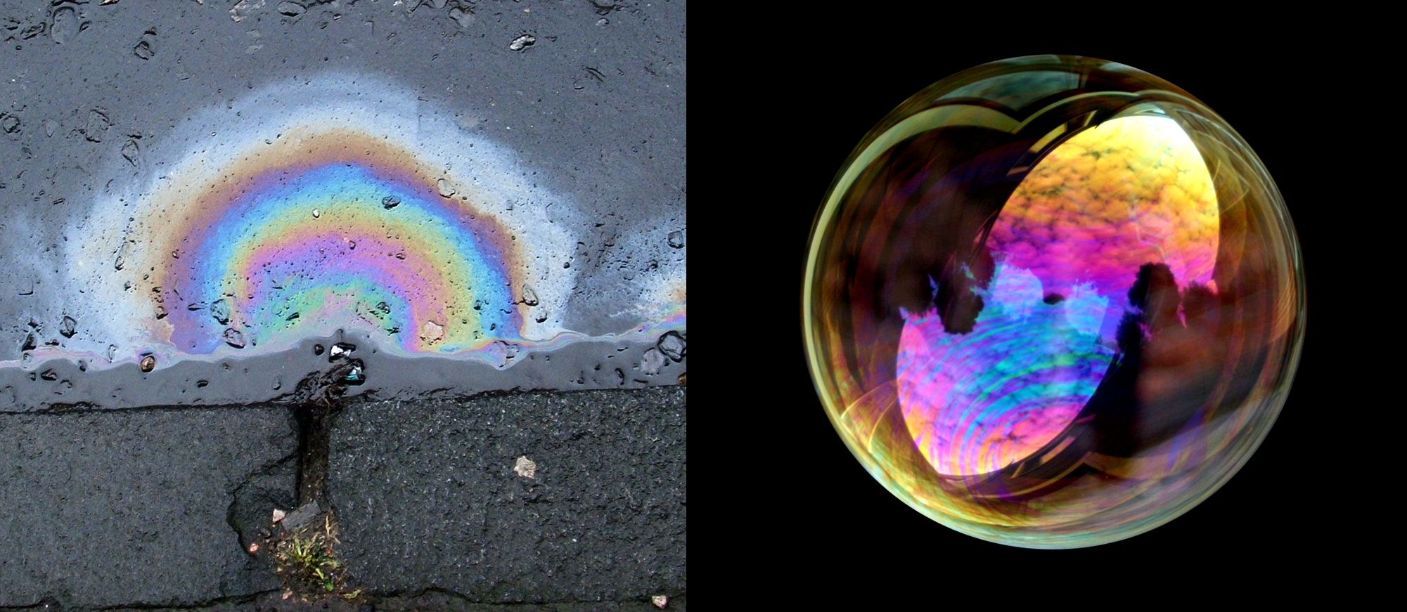
In the above summation of two fields, the resulting field follows an exact sum of the two collided fields. On the other hand, in raytracing, often, when a ray intersects with another ray, it will be left unchanged and continue its path. However, in the case of lightfields, they form a new field. This feature is called interference of light, which is not introduced in raytracing, and often raytracing omits this feature. As you can tell from also the summation, two fields could enhance the resulting field (constructive interference) by converging to a brighter intensity, or these two fields could cancel out each other (destructive interference) and lead to the absence of light --total darkness--.
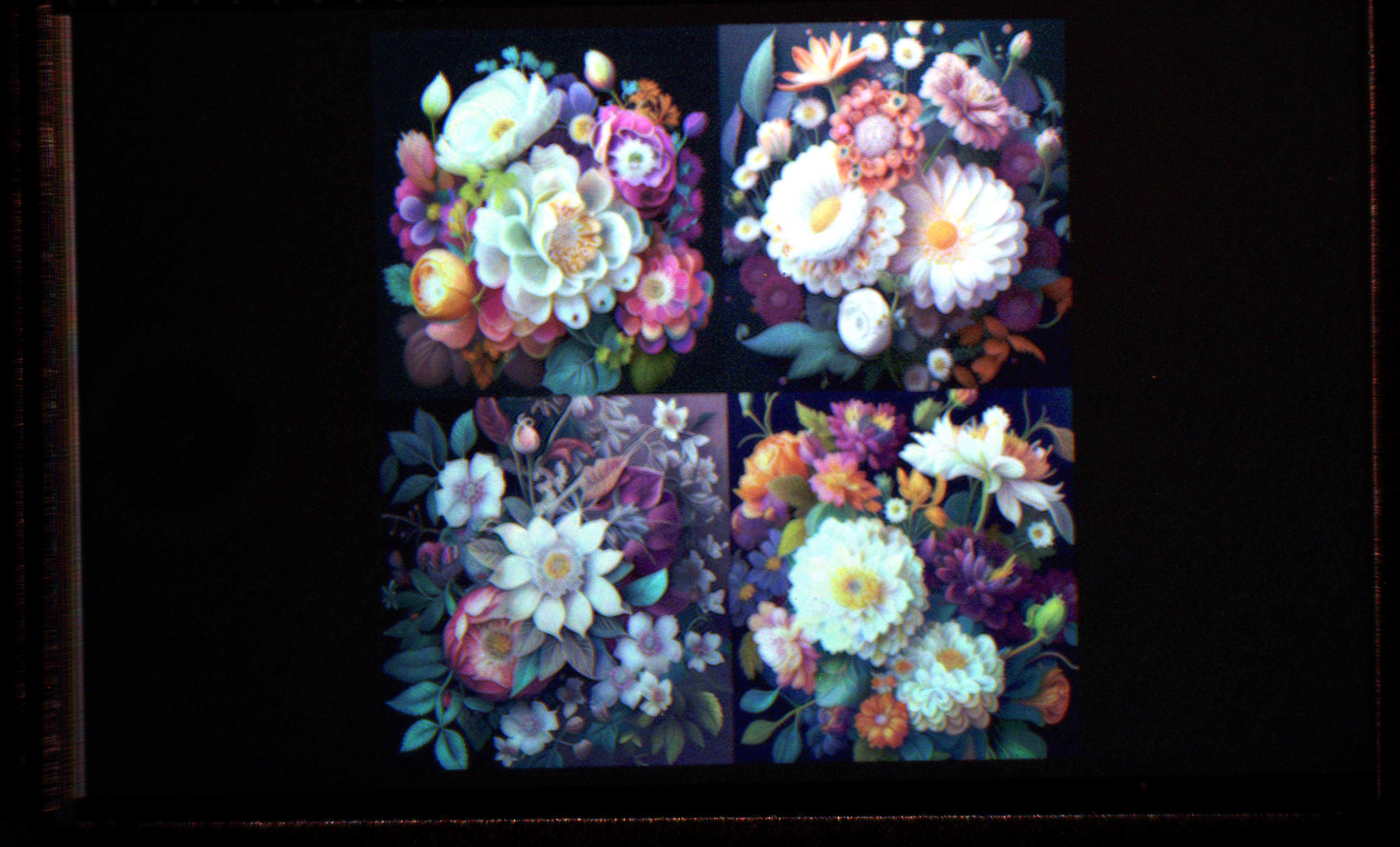
There are various examples of interference in nature. For example, the blue color of a butterfly wing results from interference, as biology typically does not produce blue-colored pigments in nature. More examples of light interference from daily lives are provided in the figure below.
We have established an easy way to describe a field with a proxy complex number form. This way, we avoided complicated trigonometric conversions. Let us look into how we use that in an actual simulation. Firstly, we can define two separate matrices to represent a field using real numbers:
import torch

amplitude = torch.tensor(100, 100, dtype = torch.float64)
phase = torch.tensor(100, 100, dtype = torch.float64)
In this above example, we define two matrices with 100 x 100 dimensions.
Each matrix holds floating point numbers, and they are real numbers.
To convert the amplitude and phase into a field, we must define the field as suggested in our previous description.
Instead of going through the same mathematical process for every piece of our future codes, we can rely on a utility function in odak to create fields consistently and coherently across all our future developments.
The utility function we will review is odak.learn.wave.generate_complex_field():
Here, we provide visual results from this piece of code as below:
Generate complex field from amplitude and phase.
Parameters:
-
amplitude–Amplitude or amplitudes. -
phase–Phase or phases in radians.
Returns:
-
field(cfloat) –Complex field or fields.
Source code in odak/learn/wave/util.py
Let us use this utility function to expand our previous code snippet and show how we can generate a complex field using that:
import torch
import odak # (1)

amplitude = torch.tensor(100, 100, dtype = torch.float64)
phase = torch.tensor(100, 100, dtype = torch.float64)
field = odak.learn.wave.generate_complex_field(amplitude, phase) # (2)
- Adding
odakto our imports. - Generating a field using
odak.learn.wave.generate_complex_field.
Propagating a field in free space 
Informative · Practical
The next question we have to ask is related to the field we generated in our previous example. In raytracing, we propagate rays in space, whereas in CGH, we propagate a field described over a surface onto another target surface. So we need a transfer function that projects our field on another target surface. That is the point where free space beam propagation comes into play. As the name implies, free space beam propagation deals with propagating light in free space from one surface to another. This entire process of propagation is also referred to as light transport in the domains of Computer Graphics. In the rest of this section, we will explore means to simulate beam propagation on a computer.
A good news for Matlab fans!
We will indeed use odak to explore beam propagation.
However, there is also a book in the literature, [Numerical simulation of optical wave propagation: With examples in MATLAB by Jason D. Schmidt](https://www.spiedigitallibrary.org/ebooks/PM/Numerical-Simulation-of-Optical-Wave-Propagation-with-Examples-in-MATLAB/eISBN-9780819483270/10.1117/3.866274?SSO=1)3, that provides a crash course on beam propagation using MATLAB.
As we revisit the field we generated in the previous subsection, we remember that our field is a pixelated 2D surface. Each pixel in our fields, either a hologram or image plane, typically has a small size of a few micrometers (e.g., \(8 \mu m\)). How light travels from each one of these pixels on one surface to pixels on another is conceptually depicted as a figure at the beginning of this section (green wolf image with two planes). We will name that figure's first plane on the left as the hologram plane and the second as the image plane. In a nutshell, the contribution of a pixel on a hologram plane could be calculated by drawing rays to every pixel on the image plane. We draw rays from a point to a plane because in wave theory --what CGH follows--, light can diffract (a small aperture creating spherical waves as Huygens suggested). Each ray will have a certain distance, thus causing various delays in phase \(\phi\). As long as the distance between planes is large enough, each ray will maintain an electric field that is in the same direction as the others (same polarization), thus able to interfere with other rays emerging from other pixels in a hologram plane. This simplified description oversimplifies solving the Maxwell equations in electromagnetics.
A simplified result of solving Maxwell's equation is commonly described using Rayleigh-Sommerfeld diffraction integrals.
For more on Rayleigh-Sommerfeld, consult Heurtley, J. C. (1973). Scalar Rayleigh–Sommerfeld and Kirchhoff diffraction integrals: a comparison of exact evaluations for axial points. JOSA, 63(8), 1003-1008. 4.
The first solution of the Rayleigh-Sommerfeld integral, also known as the Huygens-Fresnel principle, is expressed as follows:
where the field at a target image plane, \(u(x,y)\), is calculated by integrating over every point of the hologram's area, \(u_0(x,y)\). Note that, for the above equation, \(r\) represents the optical path between a selected point over a hologram and a selected point in the image plane, theta represents the angle between these two points, k represents the wavenumber (\(\frac{2\pi}{\lambda}\)) and \(\lambda\) represents the wavelength of light. In this described light transport model, optical fields, \(u_0(x,y)\) and \(u(x,y)\), are represented with a complex value,
where \(A\) represents the spatial distribution of amplitude and \(\phi\) represents the spatial distribution of phase across a hologram plane. The described holographic light transport model is often simplified into a single convolution with a fixed spatially invariant complex kernel, \(h(x,y)\) 5.
There are multiple variants of this simplified approach:
Matsushima, Kyoji, and Tomoyoshi Shimobaba. "Band-limited angular spectrum method for numerical simulation of free-space propagation in far and near fields." Optics express 17.22 (2009): 19662-19673.6,Zhang, Wenhui, Hao Zhang, and Guofan Jin. "Band-extended angular spectrum method for accurate diffraction calculation in a wide propagation range." Optics letters 45.6 (2020): 1543-1546.7,Zhang, Wenhui, Hao Zhang, and Guofan Jin. "Adaptive-sampling angular spectrum method with full utilization of space-bandwidth product." Optics Letters 45.16 (2020): 4416-4419.8.
In many cases, people choose to use the most common form of \(h(x, y)\) described as
where z represents the distance between a hologram plane and a target image plane. Before, we introduce you how to use existing beam propagation in our library, let us dive deep in compiling a beam propagation code following the Rayleigh-Sommerfeld integral, also known as the Huygens-Fresnel principle. In the rest of this script, I will walk you through the below code:
1 2 3 4 5 6 7 8 9 10 11 12 13 14 15 16 17 18 19 20 21 22 23 24 25 26 27 28 29 30 31 32 33 34 35 36 37 38 39 40 41 42 43 44 45 46 47 48 49 50 51 52 53 54 55 56 57 58 59 60 61 62 63 64 65 66 67 68 69 70 71 72 73 74 75 76 77 78 79 80 81 82 83 84 85 86 87 88 89 90 91 92 93 94 95 96 97 98 99 100 101 102 103 104 105 106 107 108 109 110 111 112 113 114 115 116 117 118 119 120 121 122 123 124 125 126 127 128 129 | |
- Importing relevant libraries
- This is our main routine.
- Length of the final image plane along X and Y axes.
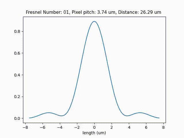
- Fresnel number is an arbitrary number that helps to get a sense if the optical configuration could be considered as a Fresnel (near field) or Fraunhofer regions.
- Propagating light with the given configuration.
- Wavelength of light.
- Square aperture length of a single pixel in the simulation. This is where light diffracts from.
- Number of pixels in the image plane along X and Y axes.
- Number of point light sources used to represent a single pixel's square aperture.
- Sample point locations along X and Y axes at the image plane.
- Sample point locations along X and Y axes at the aperture plane.
- For each, virtual point light source defined inside the aperture, we simulate the light as if divergind point light source.
- Normalize with the number of samples (trapezoid integration).
- Rest of this code is for logistics for saving images.
We start the implementation by importing necessary libraries such as odak or torch.
The first function, def main, sets the length of our image plane, where we will observe the diffraction pattern.
As we set the size of our image plane, we also set a arbitrary number called Fresnel Number,
where \(z\) is the propagation distance, \(w\) is the side length of an aperture diffracting light like a pixel's square aperture -- this is often the pixel pitch -- and \(\lambda\) is the wavelength of the light.
This number helps us to get an idea if the set optical configuration falls under a certain regime like Fresnel or Fraunhofer.
Fresnel number also provides a practical ease related to comparing solutions.
Regardless of the optical configuration, a result with a specific Fresnel number will follow a similar pattern with different optical configuration.
Thus, providing a way to verify your solutions.
In the next step, we call the light propagation function, def propagate.
In the beginning of this function, we set the optical configuration.
For instance, we set pixel_pitch, this is the side length of a square aperture that the light will diffract from.
Inside the def propagate function, we reset the distance such that it follows the input Fresnel Number and wavelength.
We define the locations of the samples across X and Y axes that will represent points to calculate on the image plane, x and y.
Than, we define the locations of the samples across X and Y axes that will represent the point light source locations inside the aperture, wxs and wys, which in this case a square aperture that represents a single pixel and its sidelength is provided by pixel_pitch.
The nested for loop goes over the wxs and wys.
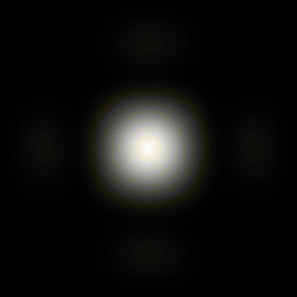
Each time, we choose a point from the aperture, we propagate a spherical wave from that point using def huygens_fresnel_principle.
Note that we accumulate the effect of each spherical wave on a variable called h.
This is diffraction pattern in complex form from our square aperture, and we also normalize it using pixel_pitch and aperture_samples.
Here, we provide visual results from this piece of code as below:
Note that beam propagation can also be learned for physical setups to avoid imperfections in a setup and to improve the image quality at an image plane:
Peng, Yifan, et al. "Neural holography with camera-in-the-loop training." ACM Transactions on Graphics (TOG) 39.6 (2020): 1-14.9,Chakravarthula, Praneeth, et al. "Learned hardware-in-the-loop phase retrieval for holographic near-eye displays." ACM Transactions on Graphics (TOG) 39.6 (2020): 1-18.10,Kavaklı, Koray, Hakan Urey, and Kaan Akşit. "Learned holographic light transport." Applied Optics (2021).11.
The above descriptions establish a mathematical understanding of beam propagation.
Let us examine the implementation of a beam propagation method called Bandlimited Angular Spectrum by reviewing these two utility functions from odak:
Helper function for odak.learn.wave.band_limited_angular_spectrum.
Parameters:
-
nu–Resolution at X axis in pixels. -
nv–Resolution at Y axis in pixels. -
dx–Pixel pitch in meters. -
wavelength–Wavelength in meters. -
distance–Distance in meters. -
device–Device, for more see torch.device().
Returns:
-
H(complex64) –Complex kernel in Fourier domain.
Source code in odak/learn/wave/classical.py
A definition to calculate bandlimited angular spectrum based beam propagation. For more
Matsushima, Kyoji, and Tomoyoshi Shimobaba. "Band-limited angular spectrum method for numerical simulation of free-space propagation in far and near fields." Optics express 17.22 (2009): 19662-19673.
Parameters:
-
field–A complex field. The expected size is [m x n]. -
k–Wave number of a wave, see odak.wave.wavenumber for more. -
distance–Propagation distance. -
dx–Size of one single pixel in the field grid (in meters). -
wavelength–Wavelength of the electric field. -
zero_padding–Zero pad in Fourier domain. -
aperture–Fourier domain aperture (e.g., pinhole in a typical holographic display). The default is one, but an aperture could be as large as input field [m x n].
Returns:
-
result(complex) –Final complex field [m x n].
Source code in odak/learn/wave/classical.py
Definitions for various beam propagation methods mostly in accordence with "Computational Fourier Optics" by David Vuelz.
Parameters:
-
field–Complex field [m x n]. -
k–Wave number of a wave, see odak.wave.wavenumber for more. -
distance–Propagation distance. -
dx–Size of one single pixel in the field grid (in meters). -
wavelength–Wavelength of the electric field. -
propagation_type(str, default:'Bandlimited Angular Spectrum') –Type of the propagation. The options are Impulse Response Fresnel, Transfer Function Fresnel, Angular Spectrum, Bandlimited Angular Spectrum, Fraunhofer. -
kernel–Custom complex kernel. -
zero_padding–Zero padding the input field if the first item in the list set True. Zero padding in the Fourier domain if the second item in the list set to True. Cropping the result with half resolution if the third item in the list is set to true. Note that in Fraunhofer propagation, setting the second item True or False will have no effect. -
aperture–Aperture at Fourier domain default:[2m x 2n], otherwise depends on `zero_padding`. If provided as a floating point 1, there will be no aperture in Fourier domain. -
scale–Resolution factor to scale generated kernel. -
samples–When using `Impulse Response Fresnel` propagation, these sample counts along X and Y will be used to represent a rectangular aperture. First two is for a hologram pixel and second two is for an image plane pixel.
Returns:
-
result(complex) –Final complex field [m x n].
Source code in odak/learn/wave/classical.py
21 22 23 24 25 26 27 28 29 30 31 32 33 34 35 36 37 38 39 40 41 42 43 44 45 46 47 48 49 50 51 52 53 54 55 56 57 58 59 60 61 62 63 64 65 66 67 68 69 70 71 72 73 74 75 76 77 78 79 80 81 82 83 84 85 86 87 88 89 90 91 92 93 94 95 96 97 98 99 100 101 102 103 104 105 106 107 108 109 110 111 112 113 114 115 116 117 118 119 120 121 122 123 124 125 126 127 128 129 130 131 132 133 134 135 136 137 138 139 140 141 142 143 144 145 146 147 148 149 150 151 | |
Let us see how we can use the given beam propagation function with an example:
import sys
import odak
import torch


def test(output_directory="test_output"):
    odak.tools.check_directory(output_directory)
    wavelength = 532e-9  # (1)
    pixel_pitch = 8e-6  # (2)
    distance = 0.5e-2  # (3)
    propagation_types = [
        "Angular Spectrum",
        "Bandlimited Angular Spectrum",
        "Transfer Function Fresnel",
    ]  # (4)
    k = odak.learn.wave.wavenumber(wavelength)  # (5)

    amplitude = torch.zeros(500, 500)
    amplitude[200:300, 200:300] = 1.0  # (5)
    phase = torch.randn_like(amplitude) * 2 * odak.pi  # (6)
    hologram = odak.learn.wave.generate_complex_field(amplitude, phase)  # (7)

    for propagation_type in propagation_types:
        image_plane = odak.learn.wave.propagate_beam(
            hologram,
            k,
            distance,
            pixel_pitch,
            wavelength,
            propagation_type,
            zero_padding=[True, False, True],  # (8)
        )  # (9)

        image_intensity = odak.learn.wave.calculate_amplitude(image_plane) ** 2  # (10)
        hologram_intensity = amplitude**2

        odak.learn.tools.save_image(
            "{}/image_intensity_{}.png".format(
                output_directory, propagation_type.replace(" ", "_")
            ),
            image_intensity,
            cmin=0.0,
            cmax=image_intensity.max(),
        )  # (11)
        odak.learn.tools.save_image(
            "{}/hologram_intensity_{}.png".format(
                output_directory, propagation_type.replace(" ", "_")
            ),
            hologram_intensity,
            cmin=0.0,
            cmax=1.0,
        )  # (12)
    assert True


if __name__ == "__main__":
    sys.exit(test())
- Setting the wavelength of light in meters. We use 532 nm (green light) in this example.
- Setting the physical size of a single pixel in our simulation. We use \(6 \mu m\) pixel size (width and height are both \(6 \mu m\).)
- Setting the distance between two planes, hologram and image plane. We set it as half a centimeterhere.
- We set the propagation type to
Bandlimited Angular Spectrum. - Here, we calculate a value named wavenumber, which we introduced while we were talking about the beam propagation functions.
- Here, we assume that there is a rectangular light at the center of our hologram.
- Here, we generate the field by combining amplitude and phase.
- Here, we zeropad and crop our field before and after the beam propagation to make sure that there is no aliasing in our results (see Nyquist criterion).
- We propagate the beam using the values and field provided.
- We calculate the final intensity on our image plane. Remember that human eyes can see intensity but not amplitude or phase of light. Intensity of light is a square of its amplitude.
- We save image plane intensity to an image file.
- For comparison, we also save the hologram intensity to an image file so that we can observe how our light transformed from one plane to another.
Let us also take a look at the saved images as a result of the above sample code:
Challenge: Light transport on Arbitrary Surfaces
We know that we can propagate a hologram to any image plane at any distance.
This propagation is a plane-to-plane interaction.
However, there may be cases where a simulation involves finding light distribution over an arbitrary surface.
Conventionally, this could be achieved by propagating the hologram to multiple different planes and picking the results from each plane on the surface of that arbitrary surface.
We challenge our readers to code the mentioned baseline (multiple planes for arbitrary surfaces) and ask them to develop a beam propagation that is less computationally expensive and works for arbitrary surfaces (e.g., tilted planes or arbitrary shapes).
This development could either rely on classical approaches or involve learning-based methods.
The resultant method could be part of odak.learn.wave submodule as a new class odak.learn.wave.propagate_arbitrary.
In addition, a unit test test/test_learn_propagate_arbitrary.py has to adopt this new class.
To add these to odak, you can rely on the pull request feature on GitHub.
You can also create a new engineering note for arbitrary surfaces in docs/notes/beam_propagation_arbitrary_surfaces.md.
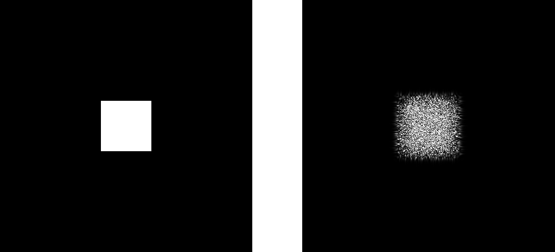
Optimizing holograms
Informative · Practical
In the previous subsection, we propagate an input field (a.k.a. lightfield, hologram) to another plane called the image plane. We can store any scene or object as a field on such planes. Thus, we have learned that we can have a plane (hologram) to capture or display a slice of a lightfield for any given scene or object. After all this introduction, it is also safe to say, regardless of hardware, holograms are the natural way to represent three-dimensional scenes, objects, and data!
Holograms come in many forms. We can broadly classify holograms as analog and digital. Analog holograms are physically tailored structures. They are typically a result of manufacturing engineered surfaces (micron or nanoscale structures). Some examples of analog holograms include diffractive optical elements 12, holographic optical elements 13, and metasurfaces 14. Here, we show an example of an analog hologram that gives us a slice of a lightfield, and we can observe the scene this way from various perspectives:
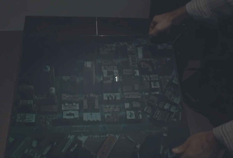
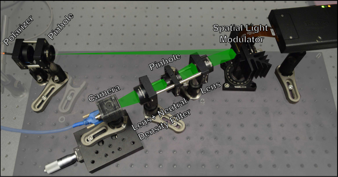
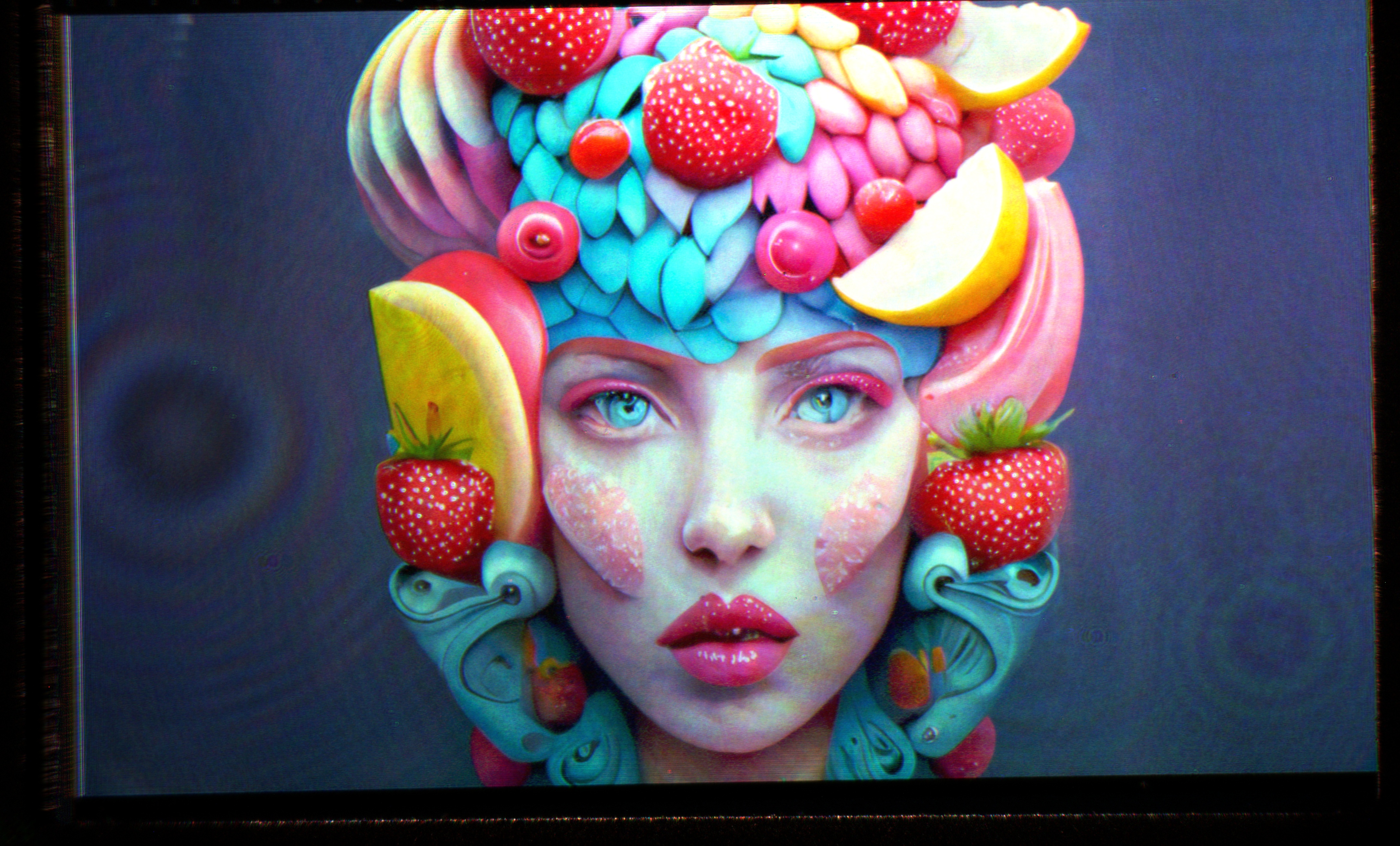
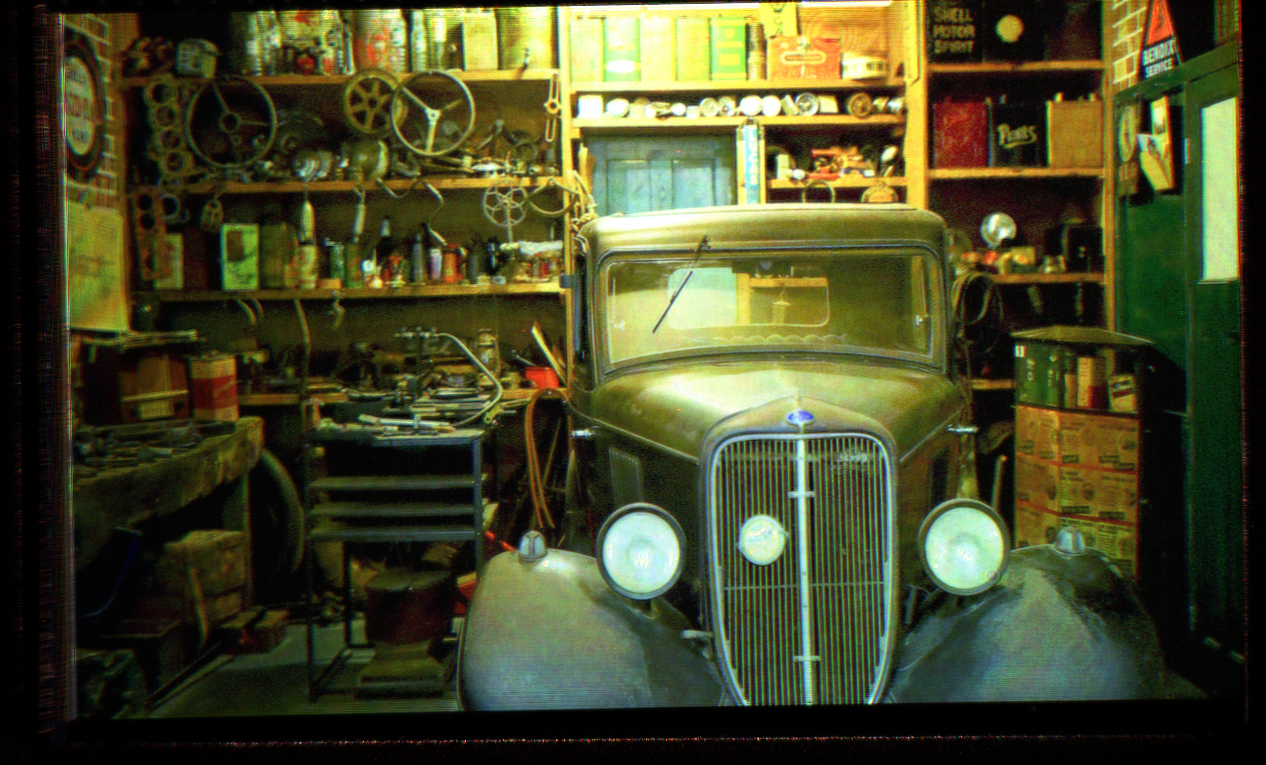
Digital holograms are the ones that are dynamic and generated using programmable versions of analog holograms. Typically, the tiniest fraction of digital holograms is a pixel that either manipulates the phase or amplitude of light. In our laboratory, we build holographic displays 15, a programmable device to display holograms. The components used in such a display are illustrated in the following rendering and contain a Spatial Light Modulator (SLM) that could display programmable holograms. Note that the SLM in this specific hardware can only manipulate phase of an incoming light.
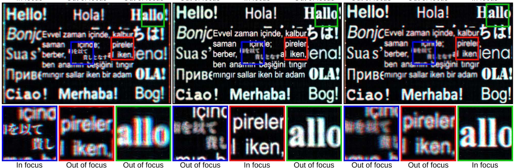
We can display holograms that generate images to fill a three-dimensional volume using the above hardware. We know that they are three-dimensional from the fact that we can focus on different parts of the images by changing the focus of our camera (closely observing the camera's location in the above figure). Let us look into a sample result to see what these three-dimensional images look like as we focus on different scene parts.
Let us look into how we can optimize a hologram for our holographic display by visiting the below example:
import sys
import odak
import torch
def test(output_directory="test_output"):
odak.tools.check_directory(output_directory)
torch.device("cpu") # (1)
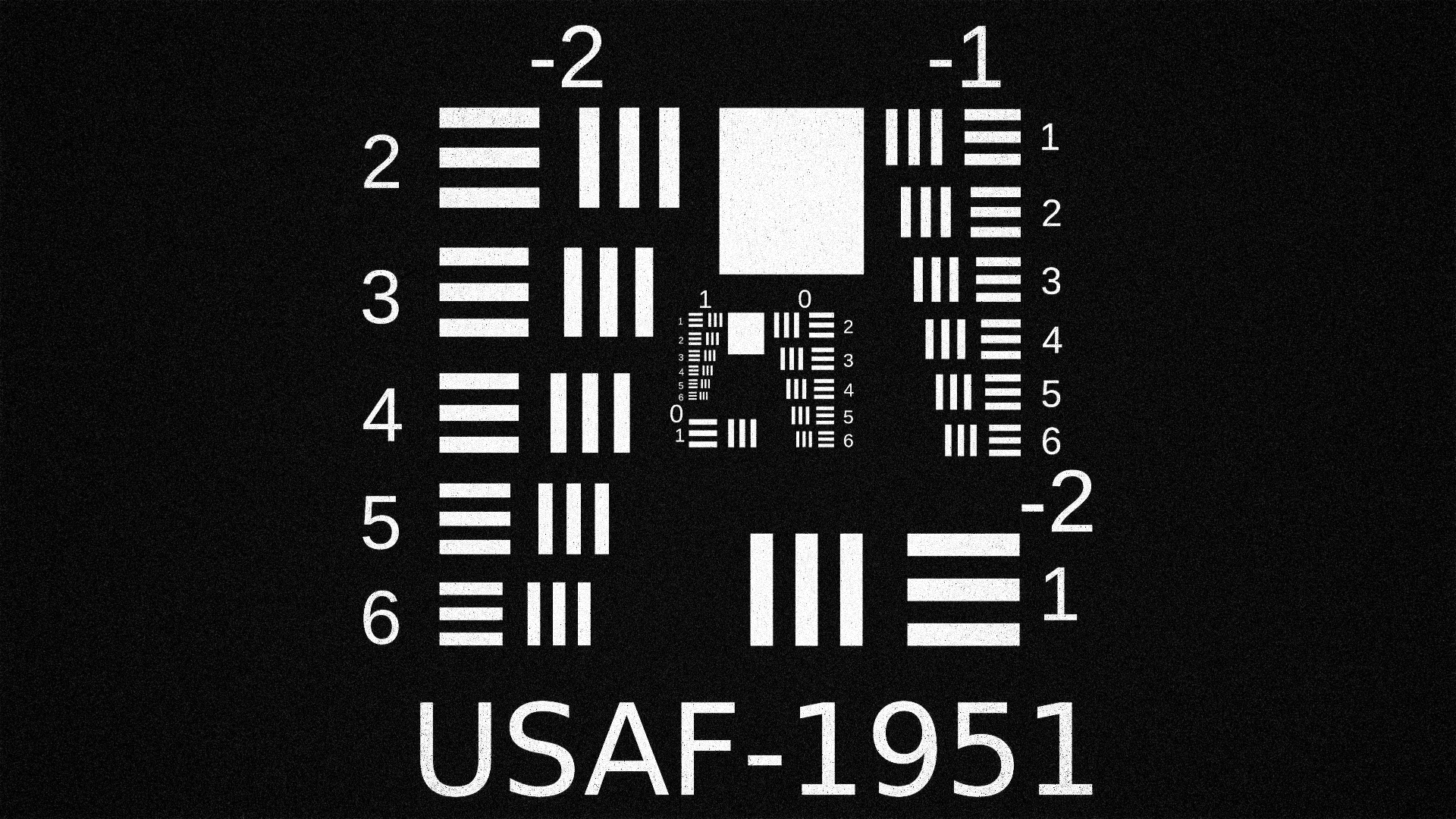
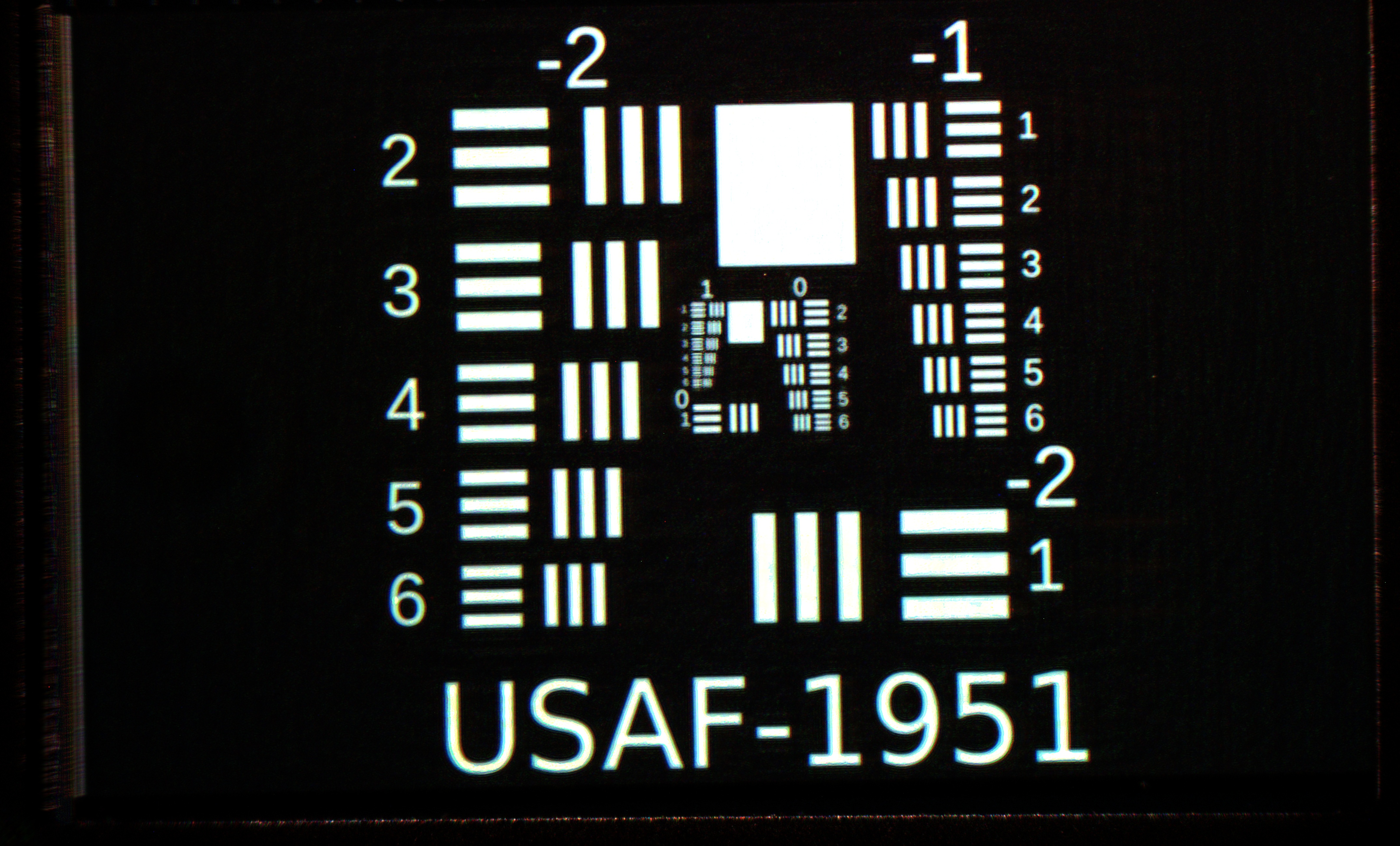
target = odak.learn.tools.load_image(
"./test/data/usaf1951.png", normalizeby=255.0, torch_style=True
)[
1
] # (4)
hologram, reconstruction = odak.learn.wave.stochastic_gradient_descent(
target,
wavelength=532e-9,
distance=20e-2,
pixel_pitch=8e-6,
propagation_type="Bandlimited Angular Spectrum",
n_iteration=50,
learning_rate=0.1,
) # (2)
odak.learn.tools.save_image(
"{}/phase.png".format(output_directory),
odak.learn.wave.calculate_phase(hologram) % (2 * odak.pi),
cmin=0.0,
cmax=2 * odak.pi,
) # (3)
odak.learn.tools.save_image(
"{}/sgd_target.png".format(output_directory), target, cmin=0.0, cmax=1.0
)
odak.learn.tools.save_image(
"{}/sgd_reconstruction.png".format(output_directory),
odak.learn.wave.calculate_amplitude(reconstruction) ** 2,
cmin=0.0,
cmax=1.0,
)
assert True
if __name__ == "__main__":
sys.exit(test())
- Replace
cpuwithcudaif you have a NVIDIA GPU with enough memory or AMD GPU with enough memory and ROCm support. - We will provide the details of this optimization function in the next part.
- Saving the phase-only hologram. Note that a phase-only hologram is between zero and two pi.
- Loading an image from a file with 1920 by 1080 resolution and using green channel.
The above sample optimization script uses a function called odak.learn.wave.stochastic_gradient_descent.
This function sits at the center of this optimization, and we have to understand what it entails by closely observing its inputs, outputs, and source code.
Let us review the function.
Definition to generate phase and reconstruction from target image via stochastic gradient descent.
Parameters:
-
target–Target field amplitude [m x n]. Keep the target values between zero and one. -
wavelength–Set if the converted array requires gradient. -
distance–Hologram plane distance wrt SLM plane. -
pixel_pitch–SLM pixel pitch in meters. -
propagation_type–Type of the propagation (see odak.learn.wave.propagate_beam()). -
n_iteration–Number of iteration. -
loss_function–If none it is set to be l2 loss. -
learning_rate–Learning rate.
Returns:
-
hologram(Tensor) –Phase only hologram as torch array
-
reconstruction_intensity(Tensor) –Reconstruction as torch array
Source code in odak/learn/wave/classical.py
1244 1245 1246 1247 1248 1249 1250 1251 1252 1253 1254 1255 1256 1257 1258 1259 1260 1261 1262 1263 1264 1265 1266 1267 1268 1269 1270 1271 1272 1273 1274 1275 1276 1277 1278 1279 1280 1281 1282 1283 1284 1285 1286 1287 1288 1289 1290 1291 1292 1293 1294 1295 1296 1297 1298 1299 1300 1301 1302 1303 1304 1305 1306 1307 1308 1309 1310 1311 1312 1313 1314 1315 1316 1317 1318 1319 1320 1321 1322 | |
Let us also examine the optimized hologram and the image that the hologram reconstructed at the image plane.
Challenge: Non-iterative Learned Hologram Calculation
We provided an overview of optimizing holograms using iterative methods.
Iterative methods are computationally expensive and unsuitable for real-time hologram generation.
We challenge our readers to derive a learned hologram generation method for multiplane images (not single-plane like in our example).
This development could either rely on classical convolutional neural networks or blend with physical priors explained in this section.
The resultant method could be part of odak.learn.wave submodule as a new class odak.learn.wave.learned_hologram.
In addition, a unit test test/test_learn_hologram.py has to adopt this new class.
To add these to odak, you can rely on the pull request feature on GitHub.
You can also create a new engineering note for arbitrary surfaces in docs/notes/learned_hologram_generation.md.
Simulating a standard holographic display 
Informative · Practical
We optimized holograms for a holographic display in the previous section. However, the beam propagation distance we used in our optimization example was large. If we were to run the same optimization for a shorter propagation distance, say not cms but mms, we would not get a decent solution. Because in an actual holographic display, there is an aperture that helps to filter out some of the light. The previous section contained an optical layout rendering of a holographic display, where this aperture is also depicted. As depicted in the rendering located in the previous section, this aperture is located between a two lens system, which is also known as 4F imaging system.
Did you know?
4F imaging system can take a Fourier transform of an input field by using physics but not computers. For more details, please review these course notes from MIT.
Let us review the class dedicated to accurately simulating a holographic display and its functions:
Internal function to reconstruct a given hologram.
Parameters:
-
hologram_phases–Hologram phases [ch x m x n]. -
amplitude–Amplitude profiles for each color primary [ch x m x n] -
no_grad–If set True, uses torch.no_grad in reconstruction. -
get_complex–If set True, reconstructor returns the complex field but not the intensities.
Returns:
-
reconstructions(tensor) –Reconstructed frames.
Source code in odak/learn/wave/propagators.py
345 346 347 348 349 350 351 352 353 354 355 356 357 358 359 360 361 362 363 364 365 366 367 368 369 370 371 372 373 374 375 376 377 378 379 380 381 382 383 384 385 386 387 388 389 390 391 392 393 394 395 396 397 398 399 400 401 402 403 404 405 406 407 408 409 410 411 412 413 414 415 416 417 418 419 420 421 422 423 424 425 426 427 428 429 430 431 432 433 | |
Function that represents the forward model in hologram optimization.
Parameters:
-
input_field–Input complex field to propagate. Shape should match the resolution configured in the propagator. -
channel_id–Index identifying the color primary (wavelength) to use for propagation. Corresponds to the index in the wavelengths list. -
depth_id–Index identifying the depth layer to propagate to. Corresponds to the index in the distances tensor. -
zero_padding_size–Target size for zero padding. If None, uses default zero padding to 2x resolution. When specified, pads the input field to this size before propagation.
Returns:
-
output_field(tensor) –Propagated output complex field at the specified depth layer. Shape matches the original input field size (cropped from padded output).
Source code in odak/learn/wave/propagators.py
263 264 265 266 267 268 269 270 271 272 273 274 275 276 277 278 279 280 281 282 283 284 285 286 287 288 289 290 291 292 293 294 295 296 297 298 299 300 301 302 303 304 305 306 307 308 309 310 311 312 313 314 315 316 317 318 319 320 321 322 323 324 325 326 327 328 329 330 331 332 333 334 335 336 337 338 339 340 341 342 343 | |
This sample unit test provides an example use case of the holographic display class.
Let us also examine how the reconstructed images look like at the image plane.

You may also be curious about how these holograms would look like in an actual holographic display, here we provide a sample gallery filled with photographs captured from our holographic display:
Conclusion
Informative
Holography offers new frontiers as an emerging method in simulating light for various applications, including displays and cameras. We provide a basic introduction to Computer-Generated Holography and a simple understanding of holographic methods. A motivated reader could scale up from this knowledge to advance concepts in displays, cameras, visual perception, optical computing, and many other light-based applications.
Reminder
We host a Slack group with more than 300 members. This Slack group focuses on the topics of rendering, perception, displays and cameras. The group is open to public and you can become a member by following this link. Readers can get in-touch with the wider community using this public group.
-
Max Born and Emil Wolf. Principles of optics: electromagnetic theory of propagation, interference and diffraction of light. Elsevier, 2013. ↩
-
Koray Kavakli, David Robert Walton, Nick Antipa, Rafał Mantiuk, Douglas Lanman, and Kaan Akşit. Optimizing vision and visuals: lectures on cameras, displays and perception. In ACM SIGGRAPH 2022 Courses, pages 1–66. 2022. ↩
-
Jason D Schmidt. Numerical simulation of optical wave propagation with examples in matlab. (No Title), 2010. ↩
-
John C Heurtley. Scalar rayleigh–sommerfeld and kirchhoff diffraction integrals: a comparison of exact evaluations for axial points. JOSA, 63(8):1003–1008, 1973. ↩
-
Maciej Sypek. Light propagation in the fresnel region. new numerical approach. Optics communications, 116(1-3):43–48, 1995. ↩
-
Kyoji Matsushima and Tomoyoshi Shimobaba. Band-limited angular spectrum method for numerical simulation of free-space propagation in far and near fields. Optics express, 17(22):19662–19673, 2009. ↩
-
Wenhui Zhang, Hao Zhang, and Guofan Jin. Band-extended angular spectrum method for accurate diffraction calculation in a wide propagation range. Optics letters, 45(6):1543–1546, 2020. ↩
-
Wenhui Zhang, Hao Zhang, and Guofan Jin. Adaptive-sampling angular spectrum method with full utilization of space-bandwidth product. Optics Letters, 45(16):4416–4419, 2020. ↩
-
Yifan Peng, Suyeon Choi, Nitish Padmanaban, and Gordon Wetzstein. Neural holography with camera-in-the-loop training. ACM Transactions on Graphics (TOG), 39(6):1–14, 2020. ↩
-
Praneeth Chakravarthula, Ethan Tseng, Tarun Srivastava, Henry Fuchs, and Felix Heide. Learned hardware-in-the-loop phase retrieval for holographic near-eye displays. ACM Transactions on Graphics (TOG), 39(6):1–18, 2020. ↩
-
Koray Kavaklı, Hakan Urey, and Kaan Akşit. Learned holographic light transport. Applied Optics, 61(5):B50–B55, 2022. ↩
-
Gary J Swanson. Binary optics technology: the theory and design of multi-level diffractive optical elements. Technical Report, MASSACHUSETTS INST OF TECH LEXINGTON LINCOLN LAB, 1989. ↩
-
Herwig Kogelnik. Coupled wave theory for thick hologram gratings. Bell System Technical Journal, 48(9):2909–2947, 1969. ↩
-
Lingling Huang, Shuang Zhang, and Thomas Zentgraf. Metasurface holography: from fundamentals to applications. Nanophotonics, 7(6):1169–1190, 2018. ↩
-
Koray Kavaklı, Yuta Itoh, Hakan Urey, and Kaan Akşit. Realistic defocus blur for multiplane computer-generated holography. In 2023 IEEE Conference Virtual Reality and 3D User Interfaces (VR), 418–426. IEEE, 2023. ↩